The S3 methods autoplot.fts() and plot.fts() are methods
for plotting results of functional two-sample tests. They visualize the
functional data and the adjusted p-values obtained from the testing
procedures for mean comparison of two groups. The plots highlight significant
effects at two levels of significance, alpha1 and alpha2, using shaded
areas.
Usage
# S3 method for class 'fts'
autoplot(
  object,
  xrange = c(0, 1),
  alpha1 = 0.05,
  alpha2 = 0.01,
  ylabel = "Functional Data",
  title = NULL,
  linewidth = 0.5,
  ...
)

# S3 method for class 'fts'
plot(
  x,
  xrange = c(0, 1),
  alpha1 = 0.05,
  alpha2 = 0.01,
  ylabel = "Functional Data",
  title = NULL,
  linewidth = 0.5,
  ...
)
Arguments
- object, x
An object of class
fts, usually a result of a call tofunctional_two_sample_test(),iwt2(),twt2(),fdr2(),pct2()orglobal2().- xrange
A length-2 numeric vector specifying the range of the x-axis for the plots. Defaults to
c(0, 1). This should match the domain of the functional data.- alpha1
A numeric value specifying the first level of significance used to select and display significant effects. Defaults to
alpha1 = 0.05.- alpha2
A numeric value specifying the second level of significance used to select and display significant effects. Defaults to
alpha2 = 0.01.- ylabel
A string specifying the label of the y-axis of the functional data plot. Defaults to
"Functional Data".- title
A string specifying the title of the functional data plot. Defaults to
NULLin which case no title is displayed.- linewidth
A numeric value specifying the width of the line for the functional data plot. Note that the line width for the adjusted p-value plot will be twice this value. Defaults to
linewidth = 0.5.- ...
Other arguments passed to specific methods. Not used in this function.
Value
The autoplot.fts() function creates a ggplot object that
displays the functional data and the adjusted p-values. The significant
intervals at levels alpha1 and alpha2 are highlighted in the plots. The
plot.fts() function is a wrapper around autoplot.fts()
that prints the plot directly.
References
Pini, A., & Vantini, S. (2017). Interval-wise testing for functional data. Journal of Nonparametric Statistics, 29(2), 407-424.
Pini, A., Vantini, S., Colosimo, B. M., & Grasso, M. (2018). Domain‐selective functional analysis of variance for supervised statistical profile monitoring of signal data. Journal of the Royal Statistical Society: Series C (Applied Statistics) 67(1), 55-81.
Abramowicz, K., Hager, C. K., Pini, A., Schelin, L., Sjostedt de Luna, S., & Vantini, S. (2018). Nonparametric inference for functional‐on‐scalar linear models applied to knee kinematic hop data after injury of the anterior cruciate ligament. Scandinavian Journal of Statistics 45(4), 1036-1061.
See also
IWTimage() for the plot of p-values heatmaps (for IWT).
Examples
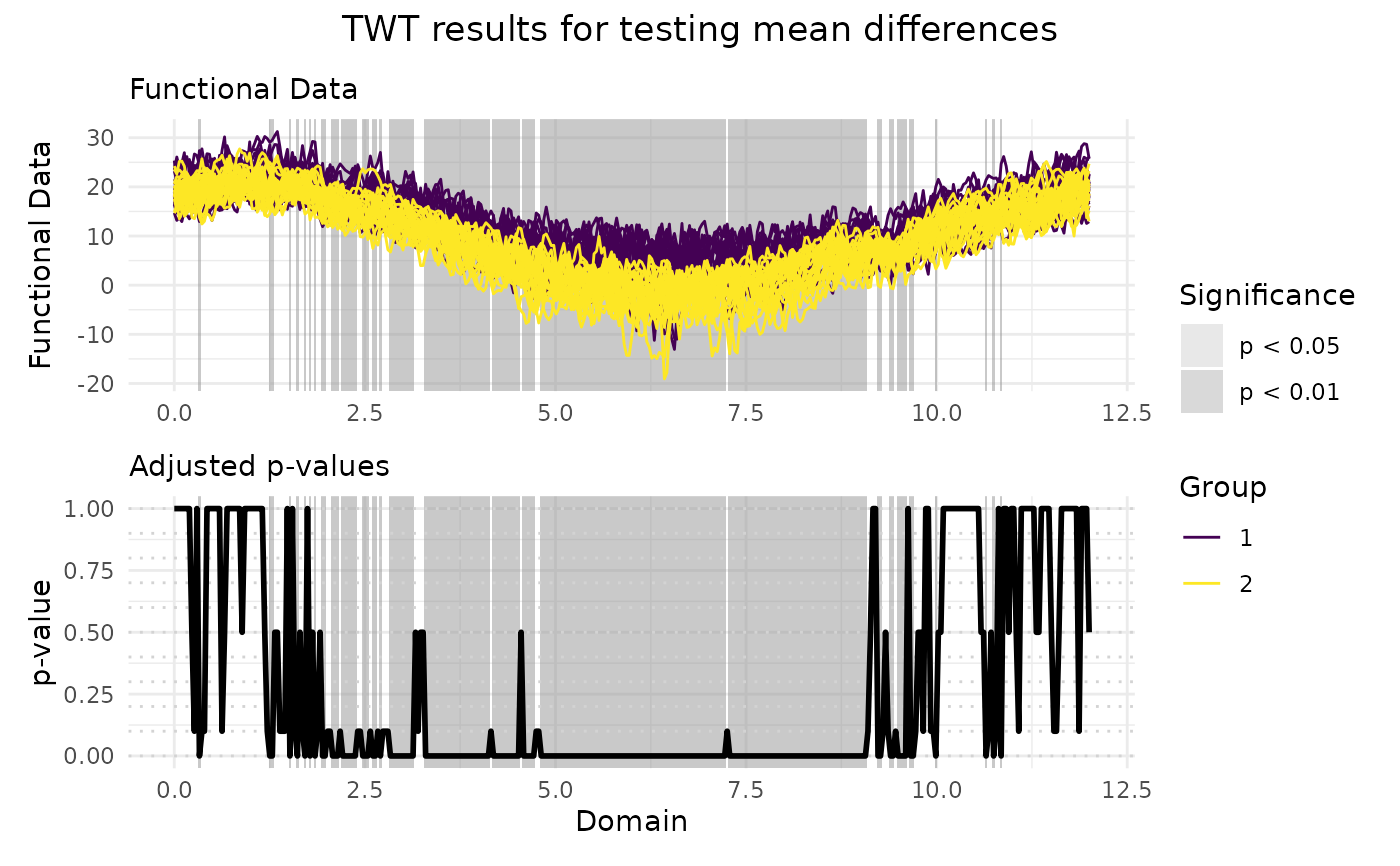
# Performing the TWT for two populations
TWT_result <- functional_two_sample_test(
NASAtemp$paris, NASAtemp$milan,
correction = "TWT", n_perm = 10L
)
# Plotting the results of the TWT
plot(
TWT_result,
xrange = c(0, 12),
title = "TWT results for testing mean differences"
)
 # Selecting the significant components at 5% level
which(TWT_result$adjusted_pval < 0.05)
#> [1] 11 39 40 47 50 53 55 57 60 61 64 65 66 68 69 70 71 72
#> [19] 73 76 77 78 80 81 83 87 88 89 90 91 92 93 94 95 96 101
#> [37] 102 103 104 105 106 107 108 109 110 111 112 113 114 115 116 117 118 119
#> [55] 120 121 122 123 124 125 126 128 129 130 131 132 133 134 135 136 137 138
#> [73] 140 141 142 143 144 147 148 149 150 151 152 153 154 155 156 157 158 159
#> [91] 160 161 162 163 164 165 166 167 168 169 170 171 172 173 174 175 176 177
#> [109] 178 179 180 181 182 183 184 185 186 187 188 189 190 191 192 193 194 195
#> [127] 196 197 198 199 200 201 202 203 204 205 206 207 208 209 210 211 212 213
#> [145] 214 215 216 217 218 219 220 222 223 224 225 226 227 228 229 230 231 232
#> [163] 233 234 235 236 237 238 239 240 241 242 243 244 245 246 247 248 249 250
#> [181] 251 252 253 254 255 256 257 258 259 260 261 262 263 264 265 266 267 268
#> [199] 269 270 271 272 273 274 275 276 281 282 286 287 289 290 291 292 294 295
#> [217] 304 324 327 330
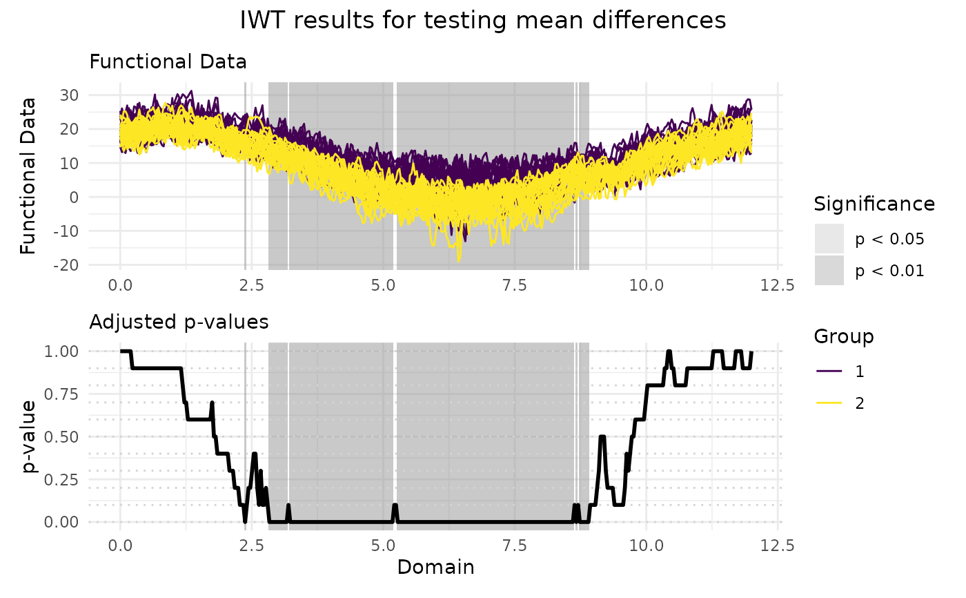
# Performing the IWT for two populations
IWT_result <- functional_two_sample_test(
NASAtemp$paris, NASAtemp$milan,
correction = "IWT", n_perm = 10L
)
# Plotting the results of the IWT
plot(
IWT_result,
xrange = c(0, 12),
title = "IWT results for testing mean differences"
)
# Selecting the significant components at 5% level
which(TWT_result$adjusted_pval < 0.05)
#> [1] 11 39 40 47 50 53 55 57 60 61 64 65 66 68 69 70 71 72
#> [19] 73 76 77 78 80 81 83 87 88 89 90 91 92 93 94 95 96 101
#> [37] 102 103 104 105 106 107 108 109 110 111 112 113 114 115 116 117 118 119
#> [55] 120 121 122 123 124 125 126 128 129 130 131 132 133 134 135 136 137 138
#> [73] 140 141 142 143 144 147 148 149 150 151 152 153 154 155 156 157 158 159
#> [91] 160 161 162 163 164 165 166 167 168 169 170 171 172 173 174 175 176 177
#> [109] 178 179 180 181 182 183 184 185 186 187 188 189 190 191 192 193 194 195
#> [127] 196 197 198 199 200 201 202 203 204 205 206 207 208 209 210 211 212 213
#> [145] 214 215 216 217 218 219 220 222 223 224 225 226 227 228 229 230 231 232
#> [163] 233 234 235 236 237 238 239 240 241 242 243 244 245 246 247 248 249 250
#> [181] 251 252 253 254 255 256 257 258 259 260 261 262 263 264 265 266 267 268
#> [199] 269 270 271 272 273 274 275 276 281 282 286 287 289 290 291 292 294 295
#> [217] 304 324 327 330
# Performing the IWT for two populations
IWT_result <- functional_two_sample_test(
NASAtemp$paris, NASAtemp$milan,
correction = "IWT", n_perm = 10L
)
# Plotting the results of the IWT
plot(
IWT_result,
xrange = c(0, 12),
title = "IWT results for testing mean differences"
)
 # Selecting the significant components at 5% level
which(IWT_result$adjusted_pval < 0.05)
#> [1] 73 87 88 89 90 91 92 93 94 95 96 97 99 100 101 102 103 104
#> [19] 105 106 107 108 109 110 111 112 113 114 115 116 117 118 119 120 121 122
#> [37] 123 124 125 126 127 128 129 130 131 132 133 134 135 136 137 138 139 140
#> [55] 141 142 143 144 145 146 147 148 149 150 151 152 153 154 155 156 157 158
#> [73] 161 162 163 164 165 166 167 168 169 170 171 172 173 174 175 176 177 178
#> [91] 179 180 181 182 183 184 185 186 187 188 189 190 191 192 193 194 195 196
#> [109] 197 198 199 200 201 202 203 204 205 206 207 208 209 210 211 212 213 214
#> [127] 215 216 217 218 219 220 221 222 223 224 225 226 227 228 229 230 231 232
#> [145] 233 234 235 236 237 238 239 240 241 242 243 244 245 246 247 248 249 250
#> [163] 251 252 253 254 255 256 257 258 259 260 261 262 264 266 267 268 269 270
#> [181] 271
# Selecting the significant components at 5% level
which(IWT_result$adjusted_pval < 0.05)
#> [1] 73 87 88 89 90 91 92 93 94 95 96 97 99 100 101 102 103 104
#> [19] 105 106 107 108 109 110 111 112 113 114 115 116 117 118 119 120 121 122
#> [37] 123 124 125 126 127 128 129 130 131 132 133 134 135 136 137 138 139 140
#> [55] 141 142 143 144 145 146 147 148 149 150 151 152 153 154 155 156 157 158
#> [73] 161 162 163 164 165 166 167 168 169 170 171 172 173 174 175 176 177 178
#> [91] 179 180 181 182 183 184 185 186 187 188 189 190 191 192 193 194 195 196
#> [109] 197 198 199 200 201 202 203 204 205 206 207 208 209 210 211 212 213 214
#> [127] 215 216 217 218 219 220 221 222 223 224 225 226 227 228 229 230 231 232
#> [145] 233 234 235 236 237 238 239 240 241 242 243 244 245 246 247 248 249 250
#> [163] 251 252 253 254 255 256 257 258 259 260 261 262 264 266 267 268 269 270
#> [181] 271