The function implements the Partition Closed Testing procedure for testing mean differences between two functional populations. Functional data are tested locally and unadjusted and adjusted p-value functions are provided. The unadjusted p-value function controls the point-wise error rate. The adjusted p-value function controls the family-wise error rate asymptotically.
Usage
pct2(
  data1,
  data2,
  partition,
  mu = 0,
  dx = NULL,
  n_perm = 1000L,
  paired = FALSE,
  alternative = c("two.sided", "less", "greater"),
  standardize = FALSE,
  verbose = FALSE,
  aggregation_strategy = c("integral", "max")
)

PCT2(
  data1,
  data2,
  partition,
  mu = 0,
  dx = NULL,
  B = 1000L,
  paired = FALSE,
  alternative = c("two.sided", "less", "greater"),
  statistic = c("Integral", "Max", "Integral_std", "Max_std"),
  verbose = FALSE
)
Arguments
- data1
Either a numeric matrix or an object of class
fda::fdspecifying the data in the first sample. If the data is provided within a matrix, it should be of shape \(n_1 \times J\) and it should contain in each row one of the \(n_1\) functions in the sample and in columns the evaluation of each function on a same uniform grid of size \(J\).- data2
Either a numeric matrix or an object of class
fda::fdspecifying the data in the second sample. If the data is provided within a matrix, it should be of shape \(n_2 \times J\) and it should contain in each row one of the \(n_2\) functions in the sample and in columns the evaluation of each function on a same uniform grid of size \(J\).- partition
An integer vector of length \(J\) specifying the membership of each point of the domain to an element of the partition. Only used and must be set if the
correctionargument is set to"PCT".- mu
Either a numeric value or a numeric vector or an object of class
fda::fdspecifying the functional mean difference under the null hypothesis. Ifmuis a constant, then a constant function is used. Ifmuis a numeric vector, it must correspond to evaluation of the mean difference function on the same grid that has been used to evaluate the data samples. Defaults to0.- dx
A numeric value specifying the step of the uniform grid on which the data are evaluated. If
NULL, the step is automatically inferred from the data. Defaults toNULL.- n_perm
An integer value specifying the number of permutations to use for the local testing procedure. Defaults to
1000L.- paired
A boolean value specifying whether a paired test should be performed. Defaults to
FALSE.- alternative
A string specifying the type of alternative hypothesis. Choices are
"two.sided","less"or"greater". Defaults to"two.sided".- standardize
A boolean value specifying whether to standardize the test statistic. Defaults to
FALSE.- verbose
A boolean value specifying whether to print the progress of the computation. Defaults to
FALSE.- aggregation_strategy
A string specifying the strategy to aggregate the point-wise test statistics for the correction procedure. Possible values are
"integral"and"max". Defaults to"integral".- B
An integer value specifying the number of permutations to use for the local testing procedure. Defaults to
1000L.- statistic
A string specifying the test statistic to use. Possible values are:
"Integral": Integral of the squared sample mean difference."Max": Maximum of the squared sample mean difference."Integral_std": Integral of the squared t-test statistic."Max_std": Maximum of the squared t-test statistic.
Defaults to
"Integral".
Value
An object of class fts containing the following components:
data: A numeric matrix of shape \(n \times J\) containing the evaluation of the \(n = n_1 + n_2\) functions on a common uniform grid of size \(p\).group_labels: An integer vector of size \(n = n_1 + n_2\) containing the group membership of each function.mu: A numeric vector of shape \(J\) containing the evaluation of the functional mean difference under the null hypothesis on the same uniform grid used to evaluate the functional samples.unadjusted_pvalues: A numeric vector of size \(J\) containing the evaluation of the unadjusted p-value function on the same uniform grid used to evaluate the functional samples.adjusted_pvalues: A numeric vector of size \(J\) containing the evaluation of the adjusted p-value functione on the same uniform grid used to evaluate the functional samples.correction_method: A string containing the correction method used to compute the adjusted p-value function.
Optionally, the list may contain the following components:
global_pvalue: A numeric value containing the global p-value. Only present if thecorrectionargument is set to"Global".pvalue_matrix: A numeric matrix of shape \(p \times p\) containing the p-values of the interval-wise tests. Element \(i, j\) contains the p-value of the test performed on the interval indexed by \(j, j+1 , \dots, j+(p-i)\). Only present if thecorrectionargument is set to"IWT".
References
Vsevolozhskaya, Olga A, Mark C Greenwood, GJ Bellante, Scott L Powell, Rick L Lawrence, and Kevin S Repasky. 2013. “Combining Functions and the Closure Principle for Performing Follow-up Tests in Functional Analysis of Variance.” Computational Statistics & Data Analysis 67: 175–84.
Vsevolozhskaya, Olga, Mark Greenwood, and Dmitri Holodov. 2014. “Pairwise comparison of treatment levels in functional analysis of variance with application to erythrocyte hemolysis.” The Annals of Applied Statistics 8 (2): 905–25. https://doi.org/10.1214/14-AOAS723.
See also
global2(), twt2(), iwt2(), fdr2() for calling directly
one of the other tests, functional_two_sample_test() for calling the
interface test and plot.fts() for plotting the results.
Examples
# Performing the PCT for two populations
# Choosing as partition the 4 seasons of the year
partition <- c(
rep(1, 31 + 28 + 21),
rep(2, 10 + 30 + 31 + 21),
rep(3, 9 + 31 + 31 + 23),
rep(4, 7 + 31 + 30 + 21),
rep(1, 10)
)
partition <- factor(partition)
PCT_result <- PCT2(NASAtemp$paris, NASAtemp$milan, partition = partition)
#> Warning: `PCT2()` was deprecated in fdatest 0.2.0.
#> ℹ Use pct2() instead. Be mindful that the argument `statistic` has been
#> replaced by `aggregation_strategy` and `standardize`.
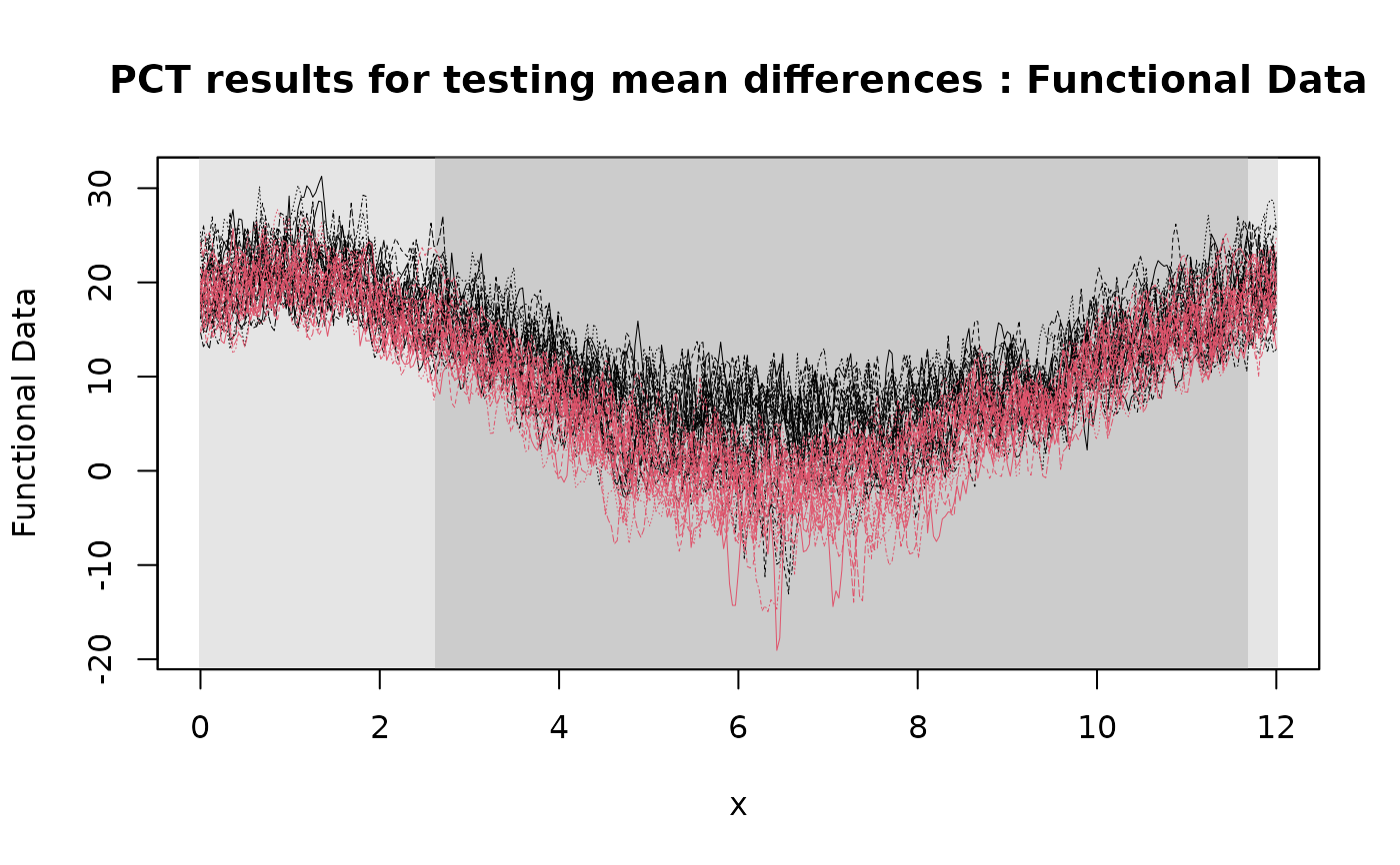
# Plotting the results of the PCT
plot(
PCT_result,
xrange = c(0, 12),
title = "PCT results for testing mean differences"
)
 # Selecting the significant components at 5% level
which(PCT_result$adjusted_pvalues < 0.05)
#> [1] 1 2 3 4 5 6 7 8 9 10 11 12 13 14 15 16 17 18
#> [19] 19 20 21 22 23 24 25 26 27 28 29 30 31 32 33 34 35 36
#> [37] 37 38 39 40 41 42 43 44 45 46 47 48 49 50 51 52 53 54
#> [55] 55 56 57 58 59 60 61 62 63 64 65 66 67 68 69 70 71 72
#> [73] 73 74 75 76 77 78 79 80 81 82 83 84 85 86 87 88 89 90
#> [91] 91 92 93 94 95 96 97 98 99 100 101 102 103 104 105 106 107 108
#> [109] 109 110 111 112 113 114 115 116 117 118 119 120 121 122 123 124 125 126
#> [127] 127 128 129 130 131 132 133 134 135 136 137 138 139 140 141 142 143 144
#> [145] 145 146 147 148 149 150 151 152 153 154 155 156 157 158 159 160 161 162
#> [163] 163 164 165 166 167 168 169 170 171 172 173 174 175 176 177 178 179 180
#> [181] 181 182 183 184 185 186 187 188 189 190 191 192 193 194 195 196 197 198
#> [199] 199 200 201 202 203 204 205 206 207 208 209 210 211 212 213 214 215 216
#> [217] 217 218 219 220 221 222 223 224 225 226 227 228 229 230 231 232 233 234
#> [235] 235 236 237 238 239 240 241 242 243 244 245 246 247 248 249 250 251 252
#> [253] 253 254 255 256 257 258 259 260 261 262 263 264 265 266 267 268 269 270
#> [271] 271 272 273 274 275 276 277 278 279 280 281 282 283 284 285 286 287 288
#> [289] 289 290 291 292 293 294 295 296 297 298 299 300 301 302 303 304 305 306
#> [307] 307 308 309 310 311 312 313 314 315 316 317 318 319 320 321 322 323 324
#> [325] 325 326 327 328 329 330 331 332 333 334 335 336 337 338 339 340 341 342
#> [343] 343 344 345 346 347 348 349 350 351 352 353 354 355 356 357 358 359 360
#> [361] 361 362 363 364 365
# Selecting the significant components at 5% level
which(PCT_result$adjusted_pvalues < 0.05)
#> [1] 1 2 3 4 5 6 7 8 9 10 11 12 13 14 15 16 17 18
#> [19] 19 20 21 22 23 24 25 26 27 28 29 30 31 32 33 34 35 36
#> [37] 37 38 39 40 41 42 43 44 45 46 47 48 49 50 51 52 53 54
#> [55] 55 56 57 58 59 60 61 62 63 64 65 66 67 68 69 70 71 72
#> [73] 73 74 75 76 77 78 79 80 81 82 83 84 85 86 87 88 89 90
#> [91] 91 92 93 94 95 96 97 98 99 100 101 102 103 104 105 106 107 108
#> [109] 109 110 111 112 113 114 115 116 117 118 119 120 121 122 123 124 125 126
#> [127] 127 128 129 130 131 132 133 134 135 136 137 138 139 140 141 142 143 144
#> [145] 145 146 147 148 149 150 151 152 153 154 155 156 157 158 159 160 161 162
#> [163] 163 164 165 166 167 168 169 170 171 172 173 174 175 176 177 178 179 180
#> [181] 181 182 183 184 185 186 187 188 189 190 191 192 193 194 195 196 197 198
#> [199] 199 200 201 202 203 204 205 206 207 208 209 210 211 212 213 214 215 216
#> [217] 217 218 219 220 221 222 223 224 225 226 227 228 229 230 231 232 233 234
#> [235] 235 236 237 238 239 240 241 242 243 244 245 246 247 248 249 250 251 252
#> [253] 253 254 255 256 257 258 259 260 261 262 263 264 265 266 267 268 269 270
#> [271] 271 272 273 274 275 276 277 278 279 280 281 282 283 284 285 286 287 288
#> [289] 289 290 291 292 293 294 295 296 297 298 299 300 301 302 303 304 305 306
#> [307] 307 308 309 310 311 312 313 314 315 316 317 318 319 320 321 322 323 324
#> [325] 325 326 327 328 329 330 331 332 333 334 335 336 337 338 339 340 341 342
#> [343] 343 344 345 346 347 348 349 350 351 352 353 354 355 356 357 358 359 360
#> [361] 361 362 363 364 365