Heatmap plot of the Interval Testing Procedure results

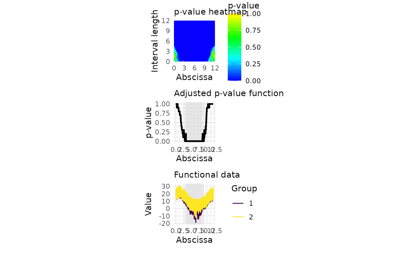
Plotting function creating a graphical output of the ITP: the p-value heat-map, the plot of the corrected p-values, and the plot of the functional data.

Usage

ITPimage(ITP_result, alpha = 0.05, abscissa_range = c(0, 1), nlevel = 20)

Arguments

ITP_result

Results of the ITP, as created by ITP1bspline, ITP1fourier, ITP2bspline, ITP2fourier, and ITP2pafourier.

alpha

Threshold for the interval-wise error rate used for the hypothesis test. The default is alpha=0.05.

abscissa_range

Range of the plot abscissa. The default is c(0,1).

nlevel

Number of desired color levels for the p-value heatmap. The default is nlevel=20.

References

A. Pini and S. Vantini (2017). The Interval Testing Procedure: Inference for Functional Data Controlling the Family Wise Error Rate on Intervals. Biometrics 73(3): 835–845.

Examples

# Performing the ITP for two populations with the B-spline basis
ITP_result <- ITP2bspline(
  NASAtemp$milan, NASAtemp$paris,
  nknots = 20,
  B = 10L
)
#> Warning: `ITP2bspline()` was deprecated in fdatest 2.2.0.
#> ℹ Please use `iwt2()` instead.

# Plotting the results of the ITP
ITPimage(ITP_result, abscissa_range=c(0,12))
#> Warning: `ITPimage()` was deprecated in fdatest 2.2.0.
#> ℹ Please use `IWTimage()` instead.


# Selecting the significant components for the radius at 5% level
which(ITP_result$corrected_pval < 0.05)
#> integer(0)