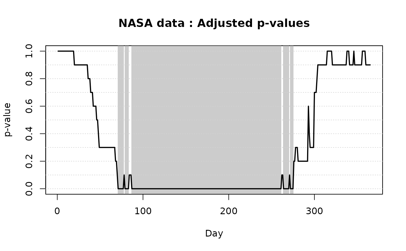
Plot method for ITP results on two-population tests

plot method for class "ITP2". Plotting function creating a graphical output of the ITP for the test of comparison between two populations: functional data and ITP-adjusted p-values are plotted.

Usage

# S3 method for class 'ITP2'
plot(
  x,
  xrange = c(0, 1),
  alpha1 = 0.05,
  alpha2 = 0.01,
  ylab = "Functional Data",
  main = NULL,
  lwd = 1,
  col = c(1, 2),
  pch = 16,
  ylim = range(object$data.eval),
  ...
)

Arguments

x

The object to be plotted. An object of class "ITP2", that is, a result of an ITP for comparison between two populations. Usually a call to ITP2bspline, ITP2fourier or ITP2pafourier.

xrange

Range of the x axis. Default is xrange=c(0,1).

alpha1

First level of significance used to select and display significant differences. Default is alpha1 = 0.05.

alpha2

Second level of significance used to select and display significant differences. Default is alpha1 = 0.01. alpha1 and alpha2 are s.t. alpha2 < alpha1. Otherwise the two values are switched.

ylab

Label of y axis of the plot of functional data. Default is "Functional Data".

main

An overall title for the plots (it will be pasted to "Functional Data" for the first plot and "adjusted p-values" for the second plot).

lwd

Line width for the plot of functional data.

col

Color used to plot the functional data.

pch

Point character for the plot of adjusted p-values.

ylim

Range of the y axis.

...

Additional plotting arguments that can be used with function plot, such as graphical parameters (see par).

Value

No value returned. The function produces a graphical output of the ITP results: the plot of the functional data and the one of the adjusted p-values. The basis components selected as significant by the test at level alpha1 and alpha2 are highlighted in the plot of the adjusted p-values and in the one of functional data (in case the test is based on a local basis, such as B-splines) by gray areas (light and dark gray, respectively). In the case of a Fourier basis with amplitude and phase decomposition, two plots of adjusted p-values are done, one for phase and one for amplitude.

References

A. Pini and S. Vantini (2017). The Interval Testing Procedure: Inference for Functional Data Controlling the Family Wise Error Rate on Intervals. Biometrics 73(3): 835–845.

Pini, A., & Vantini, S. (2017). Interval-wise testing for functional data. Journal of Nonparametric Statistics, 29(2), 407-424.

Pini, A., Vantini, S., Colosimo, B. M., & Grasso, M. (2018). Domain‐selective functional analysis of variance for supervised statistical profile monitoring of signal data. Journal of the Royal Statistical Society: Series C (Applied Statistics) 67(1), 55-81.

Abramowicz, K., Hager, C. K., Pini, A., Schelin, L., Sjostedt de Luna, S., & Vantini, S. (2018). Nonparametric inference for functional‐on‐scalar linear models applied to knee kinematic hop data after injury of the anterior cruciate ligament. Scandinavian Journal of Statistics 45(4), 1036-1061.

See also

ITPimage for the plot of p-values heatmaps. See also ITP2bspline, ITP2fourier, ITP2pafourier to perform the ITP to test for differences between two populations. See plot.ITP1 and plot.ITPlm for the plot method applied to the ITP results of one-population tests and a linear models, respectively.

Examples

# Performing the ITP for two populations with the B-spline basis
ITP.result.bspline <- ITP2bspline(
  NASAtemp$milan, NASAtemp$paris, 
  nknots = 30, B = 10L
)

# Plotting the results of the ITP
plot(
  ITP.result.bspline, 
  xlab = 'Day', 
  xrange = c(1, 365), 
  main = 'NASA data'
)



# Selecting the significant components for the radius at 5% level
which(ITP.result.bspline$adjusted.pval < 0.05)
#> integer(0)