Interval Testing Procedure for testing unctional analysis of variance with B-spline basis

The function implements the Interval Testing Procedure for testing for significant differences between several functional population evaluated on a uniform grid, in a functional analysis of variance setting. Data are represented by means of the B-spline basis and the significance of each basis coefficient is tested with an interval-wise control of the Family Wise Error Rate. The default parameters of the basis expansion lead to the piece-wise interpolating function.

Usage

ITPaovbspline(
  formula,
  order = 2,
  nknots = dim(stats::model.response(stats::model.frame(formula)))[2],
  B = 1000,
  method = "residuals"
)

Arguments

formula: An object of class "formula" (or one that can be coerced to that class): a symbolic description of the model to be fitted.
order: Order of the B-spline basis expansion. The default is order=2.
nknots: Number of knots of the B-spline basis expansion. The default is nknots=dim(data1)[2].
B: The number of iterations of the MC algorithm to evaluate the p-values of the permutation tests. The defualt is B=1000.
method: Permutation method used to calculate the p-value of permutation tests. Choose "residuals" for the permutations of residuals under the reduced model, according to the Freedman and Lane scheme, and "responses" for the permutation of the responses, according to the Manly scheme.

Value

ITPaovbspline returns an object of class "ITPaov". The function summary is used to obtain and print a summary of the results. An object of class "ITPaov" is a list containing at least the following components:

call: The matched call.
design.matrix: The design matrix of the functional-on-scalar linear model.
basis: String vector indicating the basis used for the first phase of the algorithm. In this case equal to "B-spline".
coeff: Matrix of dimensions c(n,p) of the p coefficients of the B-spline basis expansion. Rows are associated to units and columns to the basis index.
coeff.regr: Matrix of dimensions c(L+1,p) of the p coefficients of the B-spline basis expansion of the intercept (first row) and the L effects of the covariates specified in formula. Columns are associated to the basis index.
pval.F: Unadjusted p-values of the functional F-test for each basis coefficient.
pval.matrix.F: Matrix of dimensions c(p,p) of the p-values of the multivariate F-tests. The element (i,j) of matrix pval.matrix contains the p-value of the joint NPC test of the components (j,j+1,...,j+(p-i)).
adjusted.pval.F: Adjusted p-values of the functional F-test for each basis coefficient.
pval.factors: Unadjusted p-values of the functional F-tests on each factor of the analysis of variance, separately (rows) and each basis coefficient (columns).
pval.matrix.factors: Array of dimensions c(L+1,p,p) of the p-values of the multivariate F-tests on factors. The element (l,i,j) of array pval.matrix contains the p-value of the joint NPC test on factor l of the components (j,j+1,...,j+(p-i)).
adjusted.pval.factors: adjusted p-values of the functional F-tests on each factor of the analysis of variance (rows) and each basis coefficient (columns).
data.eval: Evaluation on a fine uniform grid of the functional data obtained through the basis expansion.
coeff.regr.eval: Evaluation on a fine uniform grid of the functional regression coefficients.
fitted.eval: Evaluation on a fine uniform grid of the fitted values of the functional regression.
residuals.eval: Evaluation on a fine uniform grid of the residuals of the functional regression.
R2.eval: Evaluation on a fine uniform grid of the functional R-squared of the regression.
heatmap.matrix.F: Heatmap matrix of p-values of functional F-test (used only for plots).
heatmap.matrix.factors: Heatmap matrix of p-values of functional F-tests on each factor of the analysis of variance (used only for plots).

References

A. Pini and S. Vantini (2017). The Interval Testing Procedure: Inference for Functional Data Controlling the Family Wise Error Rate on Intervals. Biometrics 73(3): 835–845.

Pini, A., Vantini, S., Colosimo, B. M., & Grasso, M. (2018). Domain‐selective functional analysis of variance for supervised statistical profile monitoring of signal data. Journal of the Royal Statistical Society: Series C (Applied Statistics) 67(1), 55-81.

Abramowicz, K., Hager, C. K., Pini, A., Schelin, L., Sjostedt de Luna, S., & Vantini, S. (2018). Nonparametric inference for functional‐on‐scalar linear models applied to knee kinematic hop data after injury of the anterior cruciate ligament. Scandinavian Journal of Statistics 45(4), 1036-1061.

D. Freedman and D. Lane (1983). A Nonstochastic Interpretation of Reported Significance Levels. Journal of Business & Economic Statistics 1.4, 292-298.

B. F. J. Manly (2006). Randomization, Bootstrap and Monte Carlo Methods in Biology. Vol. 70. CRC Press.

Examples

temperature <- rbind(NASAtemp$milan,NASAtemp$paris)
groups <- c(rep(0,22),rep(1,22))

# Performing the ITP
ITP.result <- ITPaovbspline(temperature ~ groups,B=100,nknots=20,order=3)
#> 
#> ── First step: basis expansion ─────────────────────────────────────────────────
#> Swapping 'y' and 'argvals', because 'y' is  simpler,
#>   and 'argvals' should be;  now  dim(argvals) =  365 ;  dim(y) =  365 x 44 
#> 
#> ── Second step: joint univariate tests ─────────────────────────────────────────
#> Error in eval(predvars, data, env): object 'groups' not found

# Summary of the ITP results
summary(ITP.result)
#> Error: object 'ITP.result' not found

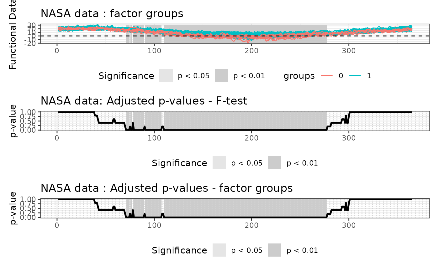
# Plot of the ITP results
graphics::layout(1)
plot(ITP.result)
#> Error: object 'ITP.result' not found

# All graphics on the same device
graphics::layout(matrix(1:4,nrow=2,byrow=FALSE))
plot(ITP.result,main='NASA data', plot.adjpval = TRUE,xlab='Day',xrange=c(1,365))
#> Error: object 'ITP.result' not found