Interval Wise Testing procedure for testing functional analysis of variance

The function implements the Interval Wise Testing procedure for testing mean differences between several functional populations in a one-way or multi-way functional analysis of variance framework. Functional data are tested locally and unadjusted and adjusted p-value functions are provided. The unadjusted p-value function controls the point-wise error rate. The adjusted p-value function controls the interval-wise error rate.

Usage

IWTaov(
  formula,
  dx = NULL,
  B = 1000L,
  method = c("residuals", "responses"),
  recycle = TRUE
)

iwt_aov(
  formula,
  dx = NULL,
  n_perm = 1000L,
  method = c("residuals", "responses"),
  recycle = TRUE
)

Arguments

formula: An object of class stats::formula (or one that can be coerced to that class) specifying the model to be fitted in a symbolic fashion. The response (left-hand side) can be either a matrix of dimension \(n \times J\) containing the pointwise evaluations of \(n\) functions on the same grid of \(J\) points, or an object of class fda::fd.
dx: A numeric value specifying the discretization step of the grid used to evaluate functional data when it is provided as objects of class fda::fd. Defaults to NULL, in which case a default value of 0.01 is used which corresponds to a grid of size 100L. Unused if functional data is provided in the form of matrices.
B: An integer value specifying the number of permutations used to evaluate the p-values of the permutation tests. Defaults to 1000L. Passed as n_perm in iwt_aov(), twt_aov() and global_aov().
method: A string specifying the permutation scheme. "residuals" permutes residuals under the reduced model (Freedman-Lane scheme); "responses" permutes the responses (Manly scheme). Defaults to "residuals".
recycle: A boolean value specifying whether the recycled version of the interval-wise testing procedure should be used. See Pini and Vantini (2017) for details. Defaults to TRUE.
n_perm: An integer value specifying the number of permutations for the permutation tests. Defaults to 1000L.

Value

An object of class faov containing the following components:

call: The matched call.
design_matrix: The design matrix of the functional ANOVA model.
unadjusted_pval_F: A numeric vector of length \(J\) containing the unadjusted p-value function of the global F-test evaluated on the grid.
adjusted_pval_F: A numeric vector of length \(J\) containing the adjusted p-value function of the global F-test evaluated on the grid.
unadjusted_pval_factors: A numeric matrix with one row per factor containing the unadjusted p-value functions of the per-factor F-tests.
adjusted_pval_factors: A numeric matrix with one row per factor containing the adjusted p-value functions of the per-factor F-tests.
data_eval: A numeric matrix containing the functional data evaluated on the grid.
coeff_regr_eval: A numeric matrix containing the functional regression coefficients evaluated on the grid.
fitted_eval: A numeric matrix containing the fitted values of the functional regression evaluated on the grid.
residuals_eval: A numeric matrix containing the residuals of the functional regression evaluated on the grid.
R2_eval: A numeric vector containing the functional R-squared evaluated on the grid.

Optionally, the list may contain the following components:

pval_matrix_F: A matrix of dimensions \(p \times p\) of p-values of the interval-wise F-tests. Element \((i,j)\) contains the p-value of the test on the interval \((j, j+1, \ldots, j+(p-i))\). Present only if correction is "IWT".
pval_matrix_factors: An array of dimensions \(L \times p \times p\) of p-values of the per-factor interval-wise F-tests. Element \((l,i,j)\) contains the p-value of the joint test on factor \(l\) and interval \((j, j+1, \ldots, j+(p-i))\). Present only if correction is "IWT".
global_pval_F: Global p-value of the overall F-test. Present only if correction is "Global".
global_pval_factors: A numeric vector of global p-values of the per-factor F-tests. Present only if correction is "Global".

References

Pini, A., & Vantini, S. (2017). Interval-wise testing for functional data. Journal of Nonparametric Statistics, 29(2), 407-424.

Pini, A., Vantini, S., Colosimo, B. M., & Grasso, M. (2018). Domain‐selective functional analysis of variance for supervised statistical profile monitoring of signal data. Journal of the Royal Statistical Society: Series C (Applied Statistics) 67(1), 55-81.

Abramowicz, K., Hager, C. K., Pini, A., Schelin, L., Sjostedt de Luna, S., & Vantini, S. (2018). Nonparametric inference for functional‐on‐scalar linear models applied to knee kinematic hop data after injury of the anterior cruciate ligament. Scandinavian Journal of Statistics 45(4), 1036-1061.

D. Freedman and D. Lane (1983). A Nonstochastic Interpretation of Reported Significance Levels. Journal of Business & Economic Statistics 1.4, 292-298.

B. F. J. Manly (2006). Randomization, Bootstrap and Monte Carlo Methods in Biology. Vol. 70. CRC Press.

Examples

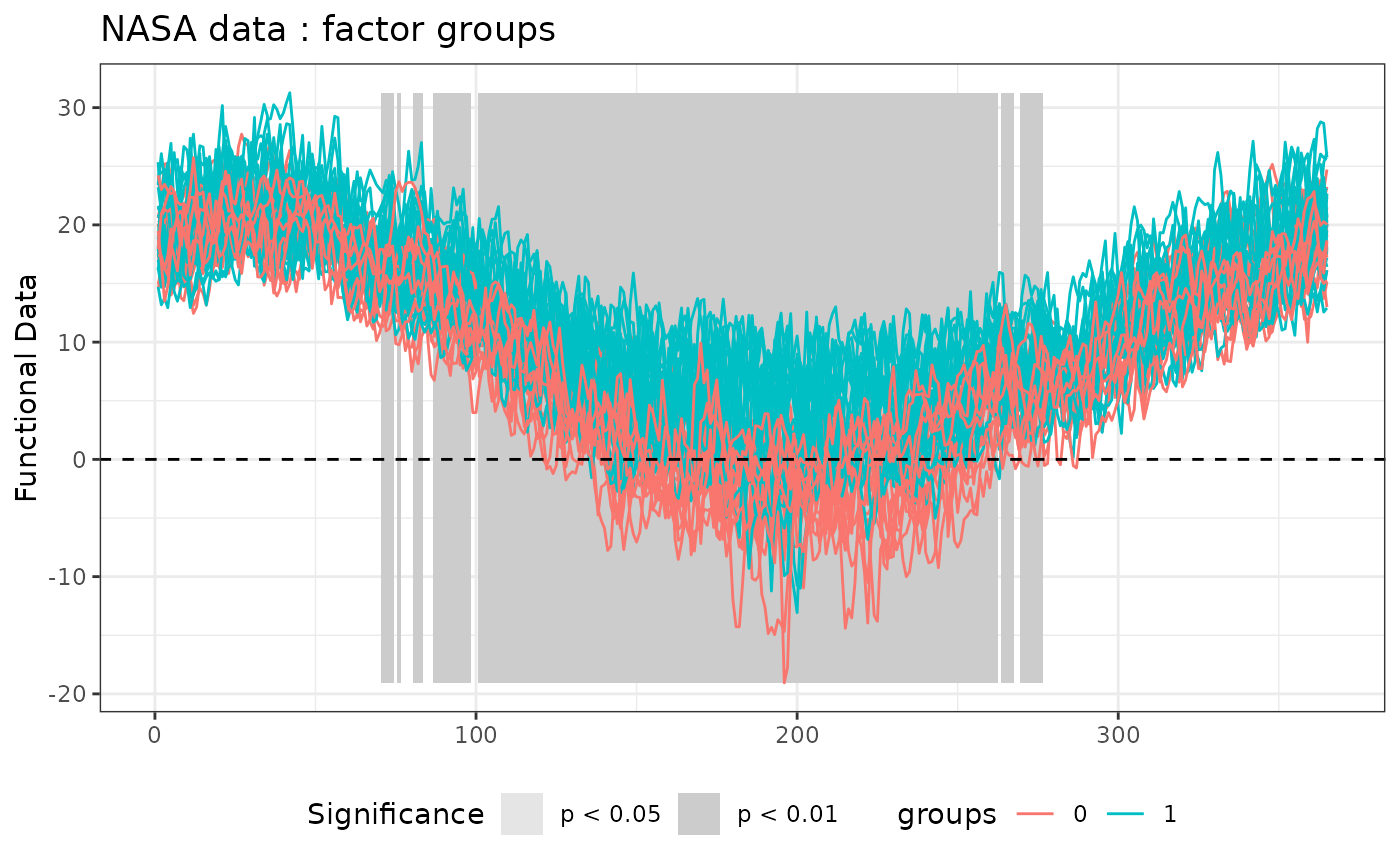
temperature <- rbind(NASAtemp$milan, NASAtemp$paris)
groups <- c(rep(0, 22), rep(1, 22))

# Performing the IWT
IWT_result <- IWTaov(temperature ~ groups, B = 10L)
#> 
#> ── Point-wise tests ────────────────────────────────────────────────────────────
#> 
#> ── Interval-wise tests ─────────────────────────────────────────────────────────
#> 
#> ── Interval-Wise Testing completed ─────────────────────────────────────────────

# Summary of the IWT results
summary(IWT_result)
#> $call
#> functional_anova_test(formula = formula, correction = "IWT", 
#>     dx = dx, B = n_perm, method = method, recycle = recycle)
#> 
#> $factors
#>        Minimum p-value    
#> groups               0 ***
#> 
#> $R2
#>               Range of functional R-squared
#> Min R-squared                  3.390203e-05
#> Max R-squared                  5.399620e-01
#> 
#> $ftest
#>   Minimum p-value    
#> 1               0 ***
#> 

# Plot of the IWT results
graphics::layout(1)
plot(IWT_result)


# All graphics on the same device
graphics::layout(matrix(1:4, nrow = 2, byrow = FALSE))
plot(
  IWT_result,
  main = "NASA data",
  plot.adjpval = TRUE,
  xlab = "Day",
  xrange = c(1, 365)
)