Plot for Functional Linear Model Test Results

The S3 methods autoplot.flm() and plot.flm() are methods for plotting results of functional-on-scalar linear model tests. They visualize the functional regression coefficients and the adjusted p-values obtained from the testing procedures. The plots highlight significant effects at two levels of significance, alpha1 and alpha2, using shaded areas.

Usage

# S3 method for class 'flm'
autoplot(
  object,
  xrange = c(0, 1),
  alpha1 = 0.05,
  alpha2 = 0.01,
  plot_adjpval = FALSE,
  col = c(1, grDevices::rainbow(dim(object$adjusted_pval_part)[1])),
  ylim = NULL,
  ylabel = "Functional Data",
  title = NULL,
  linewidth = 1,
  type = "l",
  ...
)

# S3 method for class 'flm'
plot(
  x,
  xrange = c(0, 1),
  alpha1 = 0.05,
  alpha2 = 0.01,
  plot_adjpval = FALSE,
  ylim = NULL,
  col = 1,
  ylab = "Functional Data",
  main = NULL,
  lwd = 0.5,
  type = "l",
  ...
)

Arguments

object, x: An object of class flm, usually a result of a call to functional_lm_test(), iwt_lm(), twt_lm() or global_lm().
xrange: A length-2 numeric vector specifying the range of the x-axis for the plots. Defaults to c(0, 1). This should match the domain of the functional data.
alpha1: A numeric value specifying the first level of significance used to select and display significant effects. Defaults to alpha1 = 0.05.
alpha2: A numeric value specifying the second level of significance used to select and display significant effects. Defaults to alpha2 = 0.01.
plot_adjpval: A boolean value specifying whether the plots of adjusted p-values should be displayed. Defaults to FALSE.
col: An integer specifying the color for the plot of functional data. Defaults to 1L.
ylim: A 2-length numeric vector specifying the range of the y-axis. Defaults to NULL, which determines automatically the range from functional data.
ylabel, ylab: A string specifying the label of the y-axis of the functional data plot. Defaults to "Functional Data".
title, main: A string specifying the title of the functional data plot. Defaults to NULL in which case no title is displayed.
linewidth, lwd: A numeric value specifying the width of the line for the functional data plot. Note that the line width for the adjusted p-value plot will be twice this value. Defaults to 0.5.
type: A string specifying the type of plot for the functional data. Defaults to "l" for lines.
...: Other arguments passed to specific methods. Not used in this function.

Value

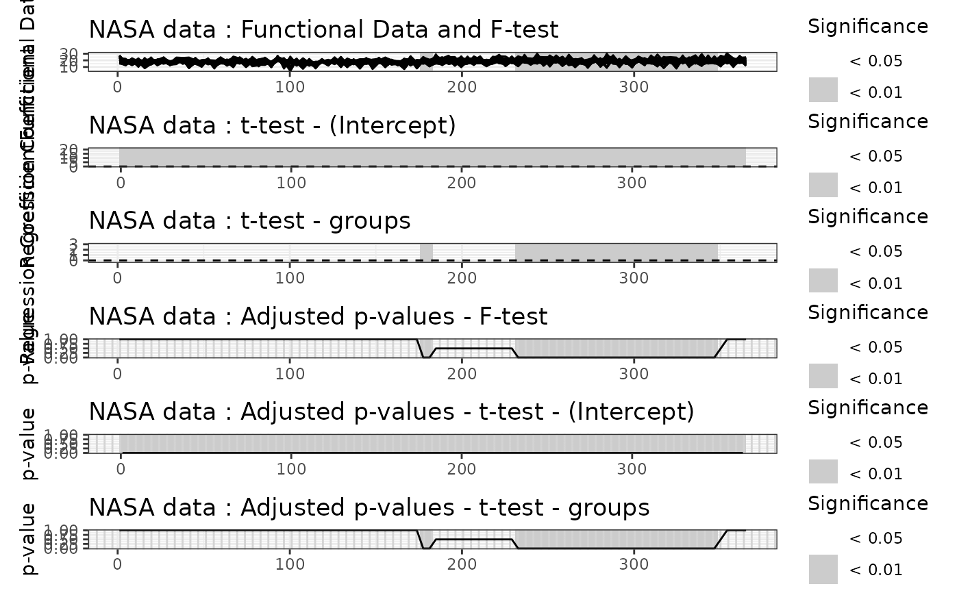
The autoplot.flm() function creates a ggplot object that displays the functional data and the adjusted p-values. The significant intervals at levels alpha1 and alpha2 are highlighted in the plots. The plot.flm() function is a wrapper around autoplot.flm() that prints the plot directly.

References

Pini, A., & Vantini, S. (2017). Interval-wise testing for functional data. Journal of Nonparametric Statistics, 29(2), 407-424.

Pini, A., Vantini, S., Colosimo, B. M., & Grasso, M. (2018). Domain‐selective functional analysis of variance for supervised statistical profile monitoring of signal data. Journal of the Royal Statistical Society: Series C (Applied Statistics) 67(1), 55-81.

Abramowicz, K., Hager, C. K., Pini, A., Schelin, L., Sjostedt de Luna, S., & Vantini, S. (2018). Nonparametric inference for functional‐on‐scalar linear models applied to knee kinematic hop data after injury of the anterior cruciate ligament. Scandinavian Journal of Statistics 45(4), 1036-1061.

Examples

temperature <- rbind(NASAtemp$milan[, 1:100], NASAtemp$paris[, 1:100])
groups <- c(rep(0, 22), rep(1, 22))

# Performing the IWT
IWT_result <- IWTlm(temperature ~ groups, B = 2L)
#> 
#> ── Point-wise tests ────────────────────────────────────────────────────────────
#> 
#> ── Interval-wise tests ─────────────────────────────────────────────────────────
#> 
#> ── Interval-Wise Testing completed ─────────────────────────────────────────────

# Summary of the IWT results
summary(IWT_result)
#> $call
#> functional_lm_test(formula = formula, correction = "IWT", dx = dx, 
#>     B = n_perm, method = method, recycle = recycle)
#> 
#> $ttest
#>             Minimum p-value    
#> (Intercept)               0 ***
#> groups                    0 ***
#> 
#> $R2
#>               Range of functional R-squared
#> Min R-squared                  0.0003189364
#> Max R-squared                  0.2476892354
#> 
#> $ftest
#>   Minimum p-value    
#> 1               0 ***
#> 

# Plot of the IWT results
plot(
  IWT_result,
  main = "NASA data",
  plot_adjpval = TRUE,
  xlab = "Day",
  xrange = c(1, 365)
)